
I am going to use four data sets to review descriptive statistics. Each data set contains winning numbers for a particular lottery in the State of New York. I got the data from data.ny.gov. Here is the list of data sets:
- Lotto: 1,750 drawings between 09/2001 and 06/2018
- Pick 10: 11,456 drawings between 01/1987 and 06/2018
- Quick Draw: 702,625 drawings between 01/2013 and 06/2018
- Take 5: 7,745 drawings between 01/1992 and 06/2018
What a great way to spend a Friday the 13th.
Lottery Drawings
Each of the four lotteries has a different kind of drawing:
- Lotto: Draw 6 numbers without replacement (1 to 59)
- Pick 10: Draw 20 numbers without replacement (1 to 80)
- Quick Draw: Draw 20 numbers without replacement (1 to 80)
- Take 5: Draw 5 numbers without replacement (1 to 39)
A given lottery consists of a draw of \(n\) objects without replacement from a population of \(N\) distinct objects. In a fair lottery, each object has an equal chance of being drawn.
Hypergeometric Distribution
The hypergeometric distribution is used when drawing without replacement. Let me first consider the simplest case. You have two kinds of objects: red and blue. Consider a population of size \(N\) with \(R\) of these being red and \(N - R\) being blue. You make a sample of size \(n\). What is the probability that there are \(r\) red objects and \(n - r\) blue objects? Out of \(N\) possible objects, the number of possible samples \(\mathcal{N}_{n}\) of size \(n\) is
Similarly, out of \(R\) red objects, the number of possible samples \(\mathcal{N}_{r}\) of size \(r\) is
For each of these \(\mathcal{N}_{r}\) ways of choosing \(r\) red objects you have \(\mathcal{N}_{n-r}\) ways of choosing \(n-r\) blue objects:
Thus, the probability that a drawing of \(n\) objects has \(r\) red ones is given by
Note that
That is, the sum of the probabilities is normalized.
Consider the special case \(R = 1\):
Then the sample either has the good object (\(r = 1\)) or it does not (\(r = 0\)). You have
or
That is, the probability for a given member of the \(N\)-population to appear in the \(n\)-sample is the corresponding fraction of the population. Another special case is \(R = r = k\) with \(1 \leq k \leq n \leq N\):
This is the familiar sampling-without-replacement probability.
Instead of good and bad objects, you have winning and non-winning numbers. Out of the \(N\) numbers, only \(n\) are winning numbers. So the probability of drawing \(n\) numbers and all of them being winning numbers is given by
For the Lotto you have
Similarly, for Take 5 you have
For Pick 10, you draw 20 numbers (out of 80) but only match 10. That is, you need to draw all 10 winning numbers besides 10 loosing numbers. The probability for this is
Note that these three probabilities are for the case of winning the jackpot.
NYS Lotto
You can load the data into a Pandas DataFrame:
import pandas as pd

df = pd.read_csv('ny-lotto.csv')
The Lotto data consists of 1,750 records with four columns:
- Draw Date
- Winning Numbers
- Bonus
- Extra
I am going to ignore the Draw Date. The Winning Numbers column has string values. The Bonus and Extra columns each have integer values. However, the Extra column only has 339 non-zero values.
Extra Column
You can extract the Extra column from the full dataframe:
extra = pd.DataFrame()
extra['Extra'] = df['Extra']
extra = extra.dropna()
The last line drops the records with missing values. A quick description is found with .describe(). From this you learn that the mean value is a bit over 31, which makes sense since the range of possible values is from 1 to 59. The minimum is 1, and the maximum is 59, which confirms that these two values were drawn at least once. More tellingly, the quartiles are close to where you expect them: 25%-quartile is between 16 and 17; 50%-quartile is 31; and the 75%-quartile is 47. If the desire is that this draw is fair and each of the 59 values is equally likely, then these statistics are promising. But due to the small size of the data, a bar chart with the counts is not very uniform:
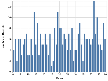
Although a few values appear less often as most values, I am not going to conclude there was any bias.
Bonus Column
You can extract the Bonus column from the full dataframe:
bonus = pd.DataFrame()
bonus['Bonus'] = df['Bonus']
Unlike the Extra column, there are no missing values in the Bonus column. A quick description is found with .describe(). From this you learn that the mean value is a bit over 30, which makes sense since the range of possible values is from 1 to 59. The minimum is 1, and the maximum is 59, which confirms that these two values were drawn at least once. More tellingly, the quartiles are right where you expect them: 25%-quartile is 15; 50%-quartile is 30; and the 75%-quartile is 45. If the desire is that this draw is fair and each of the 59 values is equally likely, then these statistics are promising. Since you have 1,750 records, the bar chart with counts is more uniform:
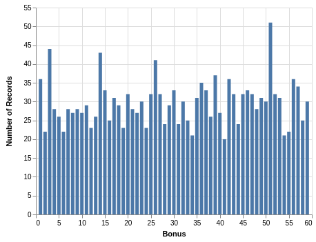
It is interesting that a number close to 50 has a higher count in both the Extra and Bonus columns.
Winning Numbers
The data in the Winning Numbers column needs to be transformed a bit:
wn = df['Winning Numbers']
wn = wn.apply(lambda x: str.split(x, ' '))
wn = wn.apply(lambda x: [int(n) for n in x])
This takes you from a string with six numbers to a list with six int values. In order to put each number drawn in its own column, I used the following:
numbers = pd.DataFrame()

for i in range(len(wn[0])):
    numbers[str(i)] = wn.apply(lambda x: x[i])
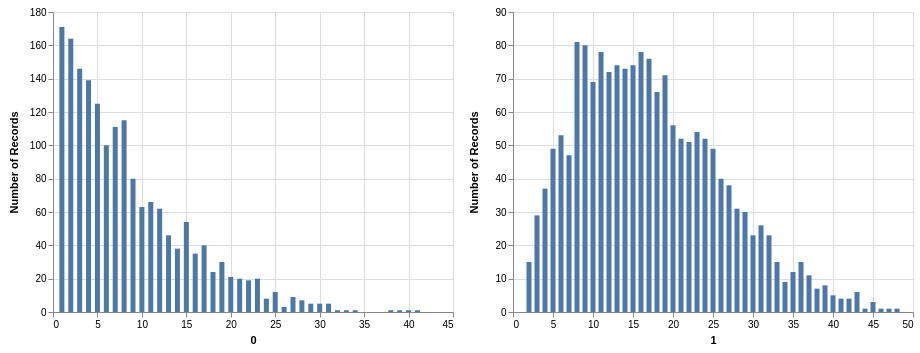
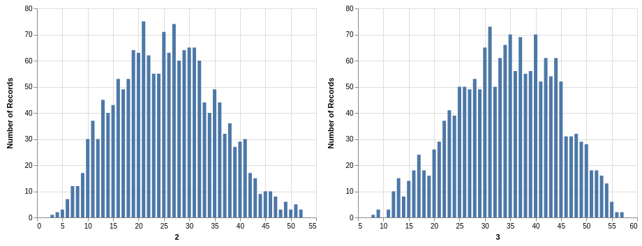
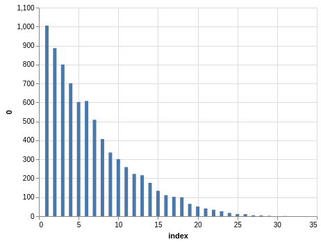
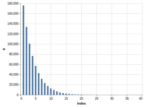
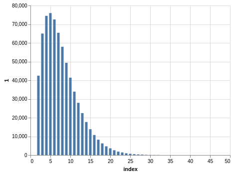
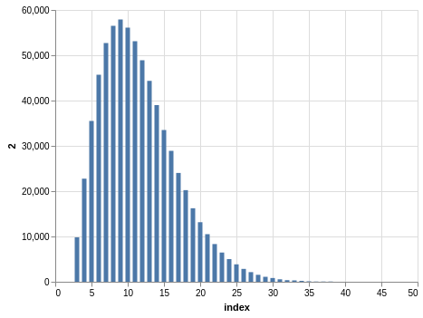
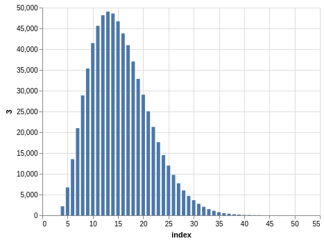
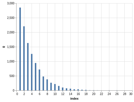
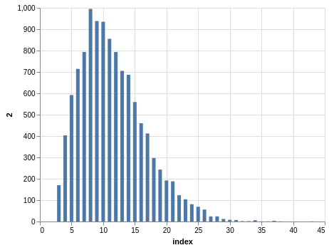
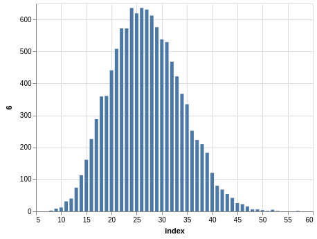
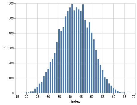
The first thing you can do is get the quick description with .describe(). But you find something interesting: There appears to be a bias in each drawing! For example, in the first drawing the mean is between 8 and 9, and the maximum is 41. Here is a bar chart with counts:
I am using Altair to produce these plots:
import altair as alt

alt.Chart(numbers).mark_bar().encode(
    alt.X(alt.repeat('column'), type='quantitative'),
    alt.Y(aggregate='count', type='quantitative'),
).repeat(
    column=['0', '1'],
)
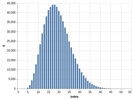
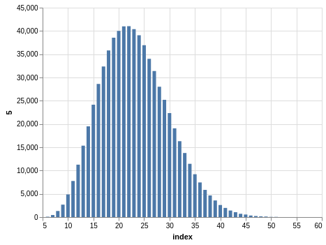
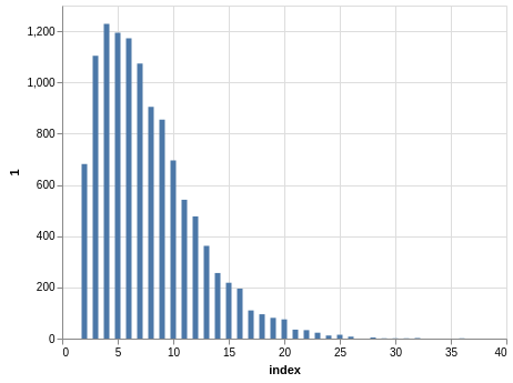
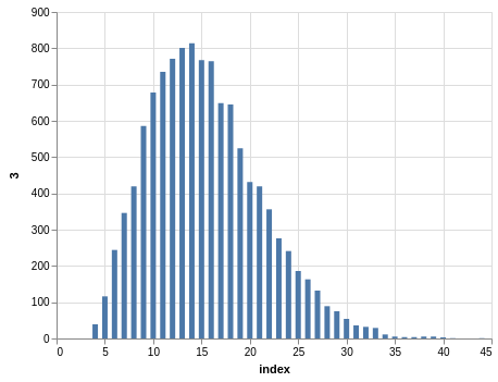
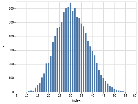
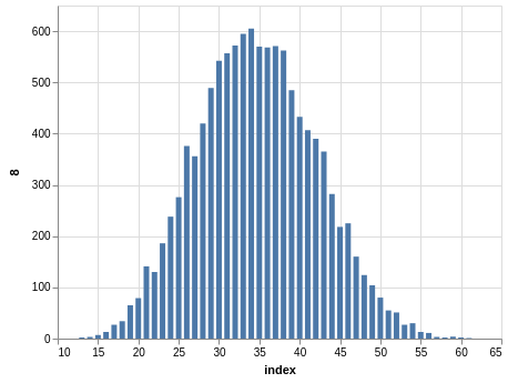
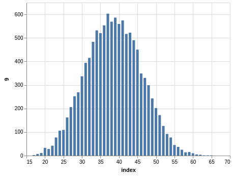
The bias is due to the fact that each sequence of winning numbers is sorted. I wish I could understand this bias better. It seems to be related to a noncentral hypergeometric distribution.
NYS Take 5
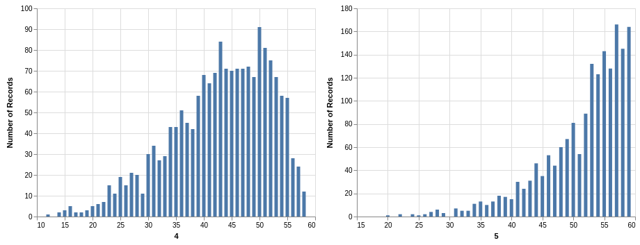
Similar steps can be taken with the Take 5 data. Here you have five winning numbers ranging from 1 to 39. Again, the winning numbers are sorted, so the bar charts with counts show a bias:
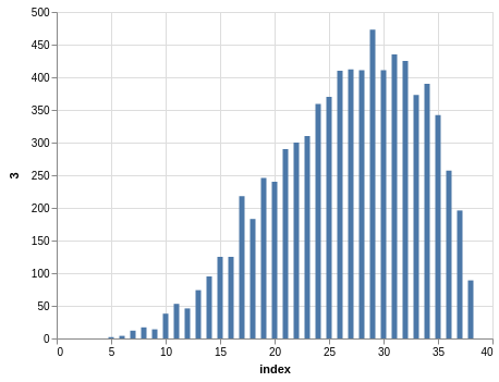
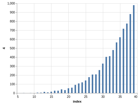
Since you have much more data than the Lotto data, the charts look smoother.
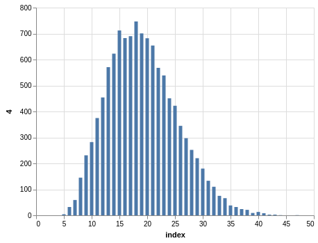
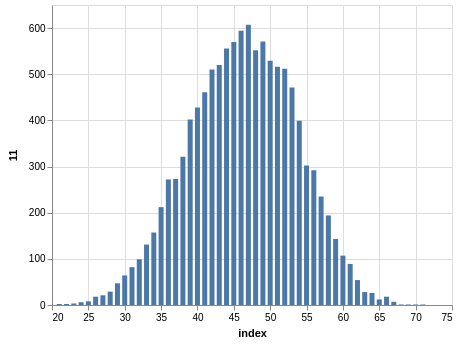
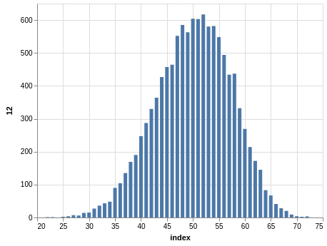
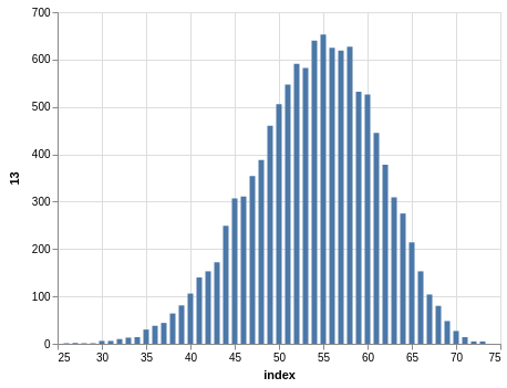
NYS Quick Draw
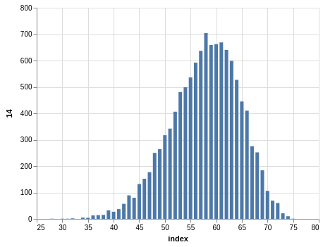
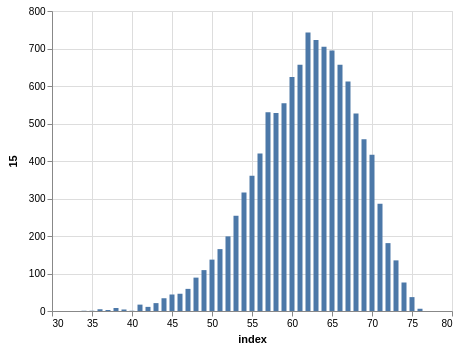
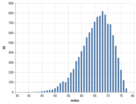
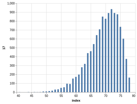
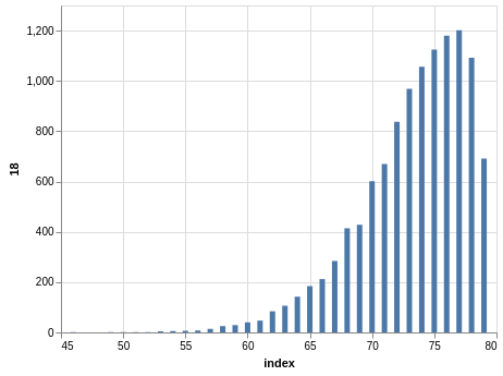
Here you have a drawing of 20 numbers ranging from 1 to 80. Again, the winning numbers are sorted, so the bar charts with the counts show a bias:
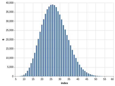
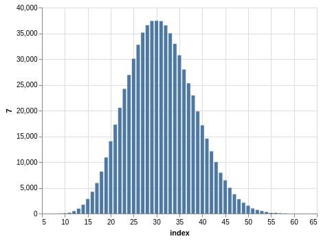
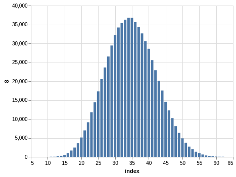
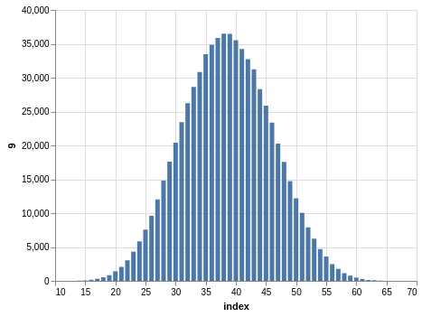
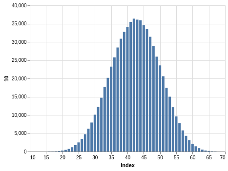
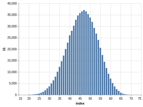
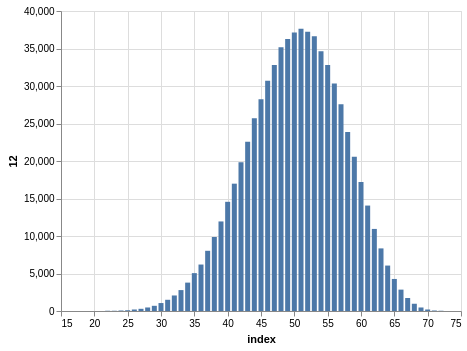
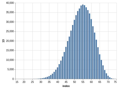
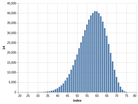
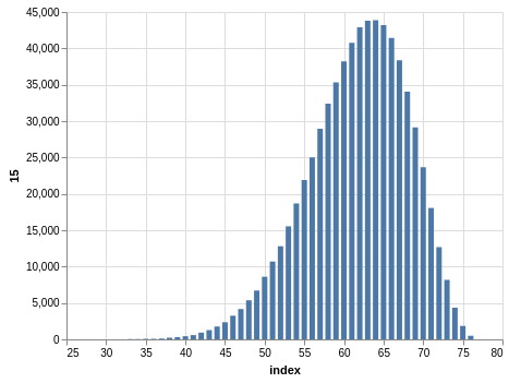
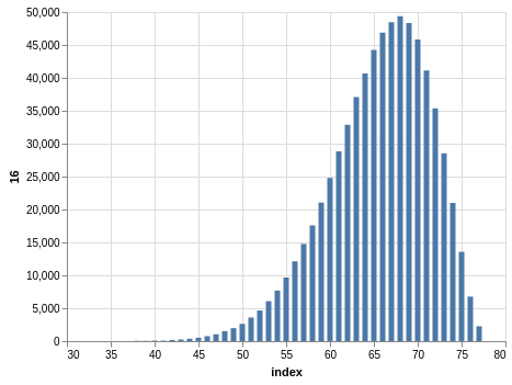
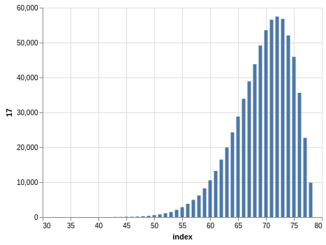
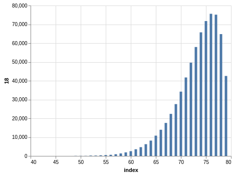
There are 702,625 records, so the charts are even smoother than the Lotto and Take 5 cases.
NYS Pick 10
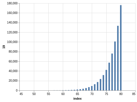
In a similar way, you can see the sorting bias in the Pick 10 data:
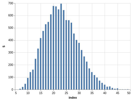
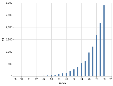
Here, you only have 11,456 records.