
There are many software libraries for deep learning. Among these, you have TensorFlow, Keras, and PyTorch. TensorFlow is the most popular one, it is developed by Google, and it is used in production code. The Torch framework is written in Lua, but PyTorch is more than just Python wrappers for Torch. The popularity of PyTorch is increasing. PyTorch is developed by Facebook. Although both PyTorch and TensorFlow are popular, they are not easy to use. Keras provides one of the easiest API to use for quick experiments. Keras can run on top of low-level libraries like TensorFlow.
Here you are going to see how to use Keras for simple regression and classification problems.
Regression
Regression is one kind of problem that can be addressed with neural networks. In this example, you are going to use concrete data from this data set. The goal is to predict the strength of the concrete from the other properties.
You can save the xls file in a directory called data. You can read the file and add it to a Pandas DataFrame via:
import pandas as pd

concrete_data = pd.read_excel("data/Concrete_Data.xls")
You can separate predictor columns and the target column as follows:
predictors = concrete_data.drop(columns='Concrete compressive strength(MPa, megapascals) ')
target = concrete_data['Concrete compressive strength(MPa, megapascals) ']
You can then split the data into training and test sets as follows:
from sklearn.model_selection import train_test_split

X_train, X_test, y_train, y_test = train_test_split(predictors, target)
The number of predicting features is found as follows:
n_cols = predictors.shape[1]
You are now ready to introduce a neural network to describe this data set. First, you import Keras:
import keras
Without any other action, you should get a message stating which backend is being used. In my case it is TensorFlow.
You can now consider the following neural network. The input layer has eight neurons, one for each feature. Then you have one hidden layer with five neurons. Then another hidden layer with five neurons. Finally the output layer with a single neuron. Each layer is dense, meaning that it connects to all the neurons in the next layer. Here are some imports:
from keras.models import Sequential
from keras.layers import Dense
You are using the Sequential model and Dense layer. The Sequential model is used when the network consist on a linear stack of layers. You define a model as follows:
model = Sequential()
Now you are ready to add layers. Here is the first hidden layer:
model.add(Dense(
    5,
    activation='relu',
    input_shape=(n_cols, ),
))
Note that the number of neurons has been specified, the activation function, and the input shape. The second hidden layer is similar:
model.add(Dense(
    5,
    activation='relu',
))
Finally, the output layer:
model.add(Dense(1))
You need to compile your model:
model.compile(
    optimizer='adam',
    loss='mean_squared_error',
)
The optimizer is how the network searches for minima. The loss specifies what kind of error function to minimize. Now you can fit your model (i.e. training):
model.fit(
    x=X_train,
x y=y_train,
    validation_data=(X_test, y_test),
    epochs=30,
)
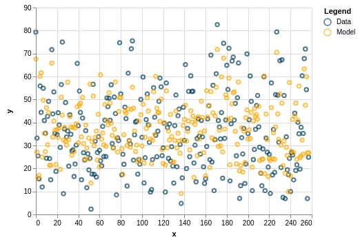
You can visualize the predictions with Altair:
import numpy as np
import altair as alt

predictions = pd.DataFrame(model.predict(X_test))

data_df = pd.DataFrame()
data_df['y'] = pd.Series(y_test.values)
data_df['x'] = pd.Series(np.arange(y_test.values.shape[0]))
data_df['Name'] = 'Data'

model_df = pd.DataFrame()
model_df['y'] = pd.Series(predictions[0])
model_df['x'] = pd.Series(np.arange(predictions.values.shape[0]))
model_df['Name'] = 'Model'

(
    alt.Chart(data_df).mark_point() +
    alt.Chart(model_df).mark_point()
).encode(
    x=alt.X(
        'x:Q',
        axis=alt.Axis(tickCount=3),
        scale=alt.Scale(zero=False),
    ),
    y=alt.Y(
        'y:Q',
        axis=alt.Axis(tickCount=4),
        scale=alt.Scale(zero=False),
    ),
    color=alt.Color(
        'Name:N',
        legend=alt.Legend(title='Legend'),
        scale=alt.Scale(
            domain=['Data', 'Model'],
            range=['#003f5c', '#ffa600'],
        ),
    ),
).save('chart.png')
Note that the result is different every time you run the model. Here is one example of modest success:
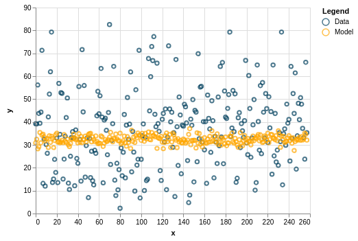
But sometimes it can be off:
Or really off:
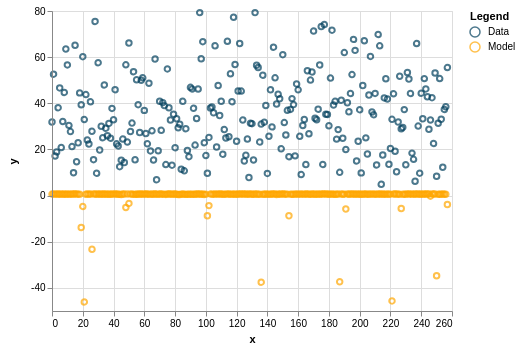
Improvements to the model include changing the amount of neurons and layers.
Classification
Classification is another kind of problem that can be solved with neural networks. You are going to use the hand-written digits data that is conveniently contained in Keras:
import keras

from keras.datasets import mnist

(X_train, y_train), (X_test, y_test) = mnist.load_data()
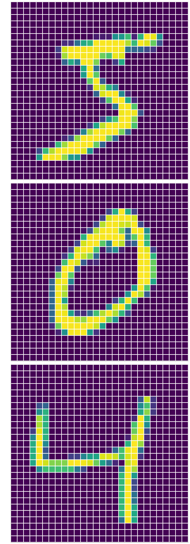
There is a simple way to visualize an example from the data set with matplotlib, but I am going to use Altair:
import numpy as np
import pandas as pd
import altair as alt

x, y = np.meshgrid(range(28), range(28))

df = pd.DataFrame()
df['x'] = pd.Series(x.ravel())
df['y'] = pd.Series(y.ravel())
df['z0'] = pd.Series(X_train[0].ravel())
df['z1'] = pd.Series(X_train[1].ravel())
df['z2'] = pd.Series(X_train[2].ravel())

chart0 = alt.Chart(df).mark_rect().encode(
    alt.X(
        'x:O',
        axis=alt.Axis(title=None, ticks=False, labels=False)
    ),
    alt.Y(
        'y:O',
        axis=alt.Axis(title=None, ticks=False, labels=False)
    ),
    alt.Color(
        'z0:Q',
        legend=None,
    ),
)

chart1 = alt.Chart(df).mark_rect().encode(
    alt.X(
        'x:O',
        axis=alt.Axis(title=None, ticks=False, labels=False)
    ),
    alt.Y(
        'y:O',
        axis=alt.Axis(title=None, ticks=False, labels=False)
    ),
    alt.Color(
        'z1:Q',
        legend=None,
    ),
)

chart2 = alt.Chart(df).mark_rect().encode(
    alt.X(
        'x:O',
        axis=alt.Axis(title=None, ticks=False, labels=False)
    ),
    alt.Y(
        'y:O',
        axis=alt.Axis(title=None, ticks=False, labels=False)
    ),
    alt.Color(
        'z2:Q',
        legend=None,
    ),
)

(chart0 & chart1 & chart2).save("color-map.png")
Here is a sample of the training data:
Here is some further pre-processing of the predictor data:
n_pixels = X_train.shape[1] * X_train.shape[2]

X_train = np.reshape(
    X_train,
    (X_train.shape[0], n_pixels),
).astype('float32')
X_test = np.reshape(
    X_test,
    (X_test.shape[0], n_pixels),
).astype('float32')

X_train = X_train / 255
X_test = X_test / 255
First, you find the total number of pixels. Then, you reshape the training and test data in order to flatten the two-dimensional image. Finally, you normalize the data. For the target data, it is important to take into account its categorical nature:
from keras.utils import to_categorical

y_train = to_categorical(y_train)
y_test = to_categorical(y_test)
This step will lead to having multiple neurons in the output layer, instead of just one.
You can figure out how many classes (or categories) there are as follows:
n_classes = y_test.shape[1]
Just as for regression, you can consider a sequential model with dense layers:
from keras.models import Sequential
from keras.layers import Dense

model = Sequential()

# First hidden layer
model.add(Dense(
    n_pixels,
    activation='relu',
    input_shape=(n_pixels,),
))

# Second hidden layer
model.add(Dense(
    100,
    activation='relu',
))

# Output layer
model.add(Dense(
    n_classes,
    activation='softmax',
))
Note that the activation function in the hidden layers is ReLU, but in the output layer it is SoftMax. This choice for the output layer will allow the results to be interpreted as probabilities.
You then compile the model:
model.compile(
    optimizer='adam',
    loss='categorical_crossentropy',
    metrics=['accuracy'],
)
Note that loss function is different now: you are using the categorical cross-entropy function. Training is as follows:
model.fit(
    X_train,
    y_train,
    validation_data=(X_test, y_test),
    epochs=10,
    verbose=2,
)
Not sure if it makes that much sense to use the test data as validation data.
Finally, you can evaluate the model:
scores = model.evaluate(X_test, y_test, verbose=0)

print(scores)
Two values are provided. The first value corresponds to the validation loss. The second value corresponds to the validation accuracy.
Models in Keras can be saved in h5 format with the save method. They can later be loaded with keras.models.load_model function.